Formulas in Ragic work similarly to those in Excel. However, Ragic's formulas are developed by us, meaning that the supported formulas or syntax may not be exactly the same. Especially, when assigning formulas, it references the Field Header directly.
Formulas can calculate not only numbers but also strings and dates. To ensure correct results, set the Field Type according to the type of calculation. For example, use a Numeric or Money field when applying numerical formulas. This allows the system to interpret the formula correctly and return the expected result. If the field type is set incorrectly, the formula may not work as intended.
To assign a formula to a Field Header from your Form Page, navigate to Design Mode and select the Field Header. Go to the Field Settings menu on the left sidebar and enter your formula into the Formula tab.
For example, in the "Sales Order" sheet, if the formula for the "Amount Due" field (A20) is "Total (A17) + Tax (A19)", you would enter "A17+A19" in that cell. Note that the formula should reference the location of the field headers.
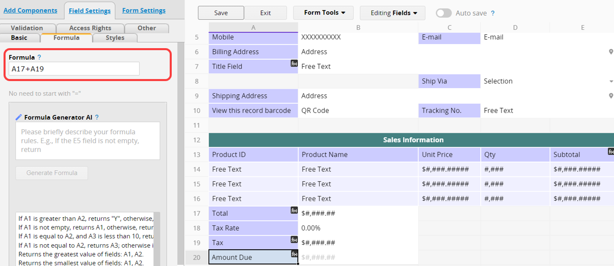
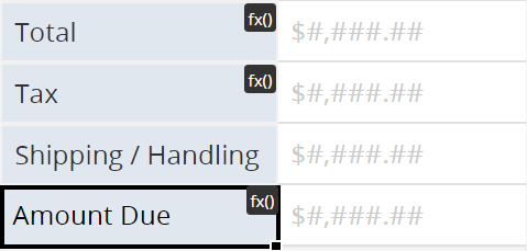
There is a fx() icon in the field assigned with the formula.
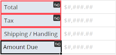
Clicking on the icon, the system will automatically highlight all the referenced fields of this formula.
For the list of supported formulas in Ragic, please refer here.
Note: The Multiple Select Field Type can only apply specific formulas from the list.
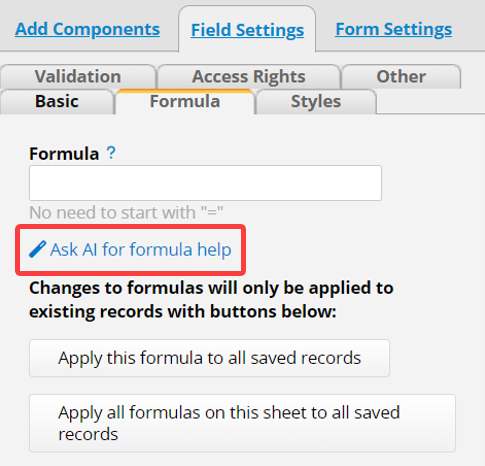
When you don't know how to create formulas, you can specify the rule you want in the Formula Generator. Let AI help you generate it.
Note: On-premises Private Server require a parameter to enable this feature. See this section for details.
Please note:
1. Describe the rules and specify the expected return value for this field. For example: Return today's date.
2. If you want to include text in your formula, enclose it in double quotation marks. For example: "Transaction Date".
3. After configuring the formula, please manually verify whether the results meet the expected outcomes.
To open the Formula Generator interface, click on the Ask AI for formula help below.
Input rules and click Generate Formula.
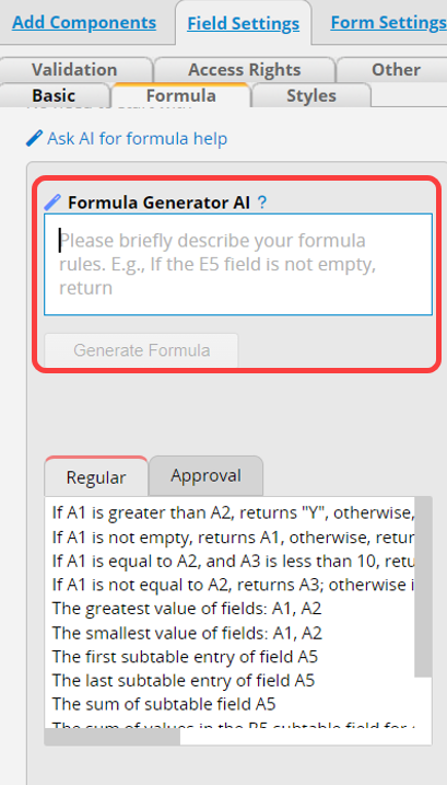
Below are some default scenarios you can select and enter the fields based on your sheet, including Regular formulas and Approval formulas.
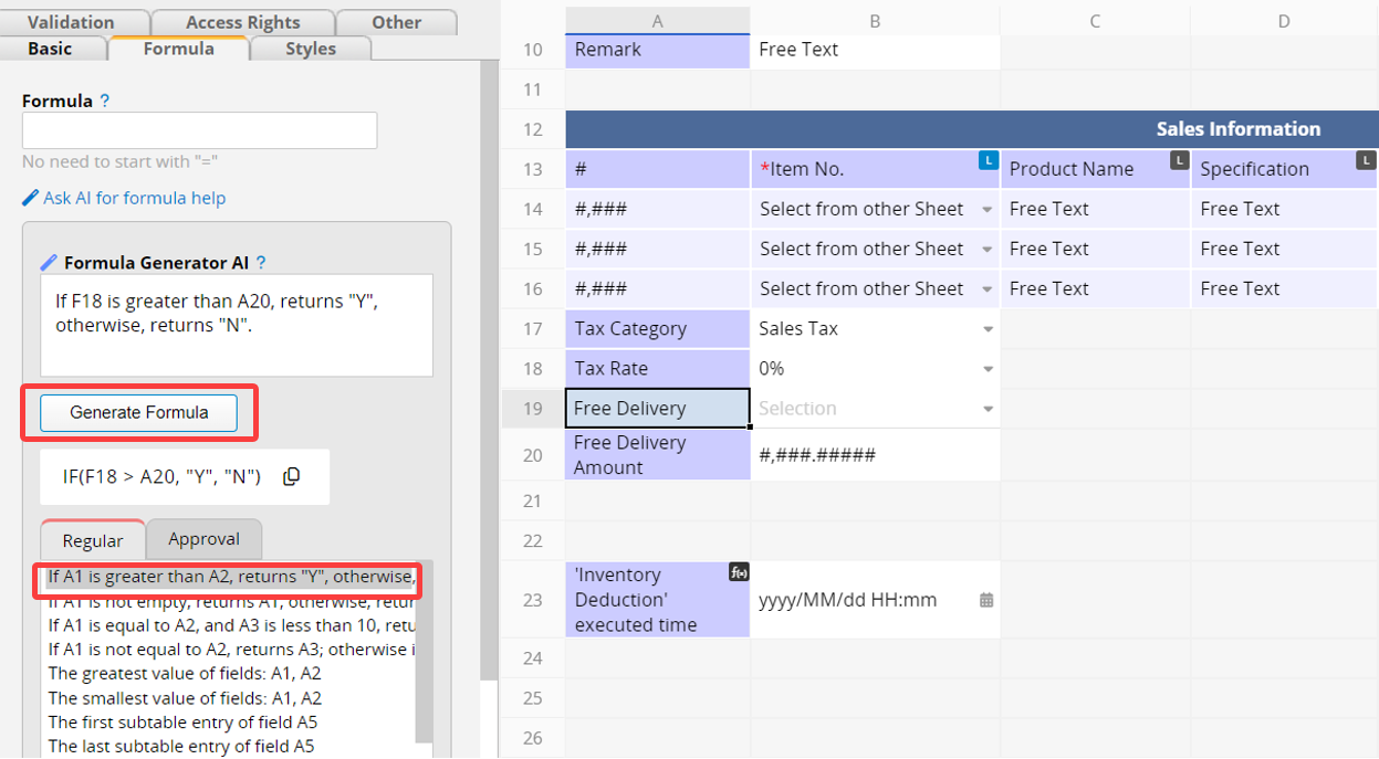
For example, if you want the "Free Delivery" field to return "Yes" when the "Total" is greater than the "Free Delivery Amount," and "No" otherwise, you can choose "If A1 is greater than A2, return 'Y', otherwise return 'N'," and then modify it to match the relevant fields and return values.
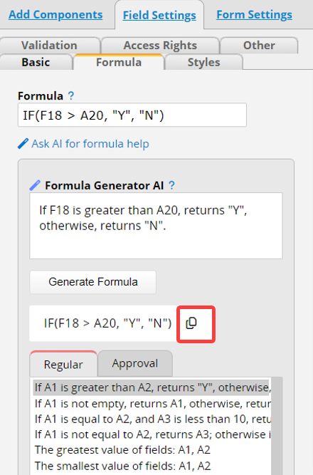
After completing, click Generate Formula to generate the corresponding formula below. Click the "copy" icon next to the formula to automatically input the formula.
Operators specify the type of calculation that you want to perform on the arguments of a formula. There is a default order in which calculations are programmed to occur, but you can change this order by using "parentheses ()".
Note: Unlike Excel, Ragic does not allow a colon ":" to be used as a reference operator to combine ranges of cells.
To perform basic mathematical operations such as addition, subtraction, or multiplication and produce numeric results, please use the following arithmetic operators:
| Arithmetic operator | Meaning | Example |
|---|---|---|
| + (plus sign) | Addition | 3+3 |
| – (minus sign) | Subtraction | 3–1 |
| * (asterisk) | Multiplication | 3*3 |
| / (forward slash) | Division | 3/3 |
| ^ (caret) | Exponentiation | 3^2 |
You can compare two values with the following operators. When two values are compared by using these operators, the result is a logical value either TRUE or FALSE that can be used within Conditional Formulas.
| Comparison operator | Meaning | Example |
|---|---|---|
| = | Equal to | A1=B1 |
| == | Equal to | A1==B1 |
| > | Greater than | A1 > B1 |
| < | Less than | A1 < B1 |
| > = | Greater than or equal to | A1 > =B1 |
| < = | Less than or equal to | A1 < =B1 |
| != | Not equal to | IF(A1!=B1,'yes','no') |
| <> | Not equal to | IF(A1<>B1,'yes','no') |
To create strings in formulas, you can use either 'single quotes', or "double quotes". In this document, we will use 'single quotes' for consistency, but both formats are acceptable in Ragic.
The following lists all formula categories supported in Ragic. You can refer to each category for detailed formulas and usage examples as needed. Please note that the following formulas are case-sensitive.
1. Numeric Calculation Formulas
6. Multiple Select Field Formulas
Formulas for calculating numerical values and amounts, such as obtaining sums, averages, maximum and minimum values, etc. For detailed explanations, please refer to this section.
| Formula | Description |
|---|---|
| SUM(value1,[value2],...) | Returns the sum of (adds) all the field values. You can also directly use the format value+value2+...to represent it. |
| AVG(value1, value2,...) | Returns the average (arithmetic mean) of all the listed field values. Note that this function also works for Subtables, where the average of all referenced field values will be added to the calculation. It works the same as the AVERAGE function. |
| AVERAGE(value1, value2,...) | Returns the average (arithmetic mean) of all the listed field values. Note that this function also works for Subtables, where the average of all referenced field values will be added to the calculation. It works the same as the AVG function. |
| MIN(value) | Returns the smallest number in a set of field values. This function also works for Subtables. |
| MAX(value) | Returns the largest numeric value in a range of field values. This function also works for Subtables. |
| MODE.SNGL(value1,[value2],...) | Returns the most common value in a range of field values. This function works for independent fields, Subtables, and global constants. |
| MODE.MULT(value1,[value2],...) | Returns multiple most common values in a range of field values. This function works for independent fields, Subtables, and global constants. |
| ABS(value) | Returns the absolute value of a number. The absolute value of a number is the number without its sign. |
| CEILING(value,[significance]) | Rounds number up, away from zero, to the nearest multiple of significance. Significance is optional; if not specified, round up to the nearest integer. Example: CEILING(2.5) will return 3; CEILING(1.5, 0.1) will return 1.5. |
| FLOOR(value,[significance]) | Rounds number down, toward zero, to the nearest multiple of significance. Significance is optional; if not specified, round down to the nearest integer. Example: FLOOR(2.5) will return 2; FLOOR(1.58, 0.1) will return 1.5. |
| ROUND(value) | Rounds a number to the nearest integer. |
| ROUND(value,N) | Rounds a number to N decimal place. |
| ROUNDUP(value,N) | Rounds up a number (away from zero) to N decimal place. |
| ROUNDDOWN(value,N) | Rounds down a number (toward zero) to N decimal place. |
| MROUND(number,N) | Rounds a number to the nearest multiple of N |
| SQRT(value) | Returns the square root of a number. |
| COUNT(value1,value2,...) | Returns the total number of field values. Empty values will not be counted when referencing independent fields but will be counted when referencing Subtable fields. |
| PI() | Returns the number 3.14159265358979, the mathematical constant pi, and the ratio of the circumference of a circle to its diameter, accurate to 15 digits. |
| RAND() | Returns an evenly distributed random real number greater than or equal to 0 and less than 1. A new random real number is returned every time the worksheet is calculated. For details, click here. |
| POWER(value,power) | Returns the result of a number value raised to a power. |
| MOD(value,divisor) | Returns the remainder after a number value is divided by a divisor. The result has the same sign as the divisor. For details, click here. |
| GCD(value1,[value2],...) | Returns the greatest common divisor of two or more integers. The greatest common divisor is the largest integer that divides the specified number of values without a remainder. For details, click here. |
| LCM(value1,[value2],...) | Returns the least common multiple of integers. The least common multiple is the smallest positive integer, which is a multiple of all integer arguments value1, value2, and so on. Use LCM to add fractions with different denominators. For details, click here. |
| PRODUCT() | Multiplies all the numerical values in referenced fields (neglecting empty and text values). You can also reference a Subtable field to multiply all the numeric values of that field. For details, click here. |
| PMT(rate, nper, pv, [fv], [type]) | Calculates the payment for a loan. For details, click here. |
Formulas for obtaining date and time-related data, such as returning the year, month, day, time, or specific workdays. For detailed explanations, please refer to this section.
| Formula | Description |
|---|---|
| TODAY() | Returns the current date. In case of automatic daily recalculation, please replace TODAY() with TODAYTZ(). |
| TODAYTZ() | Returns the current date according to Company Local Time Zone in your Account Settings. |
| NOW() | Returns the current date and time. |
| NOWTZ() | Returns the current date and time according to the Company Local Time Zone in your Account Settings. |
| EDATE(start_date, months) | Returns the serial number that represents the date that is the indicated number of months before or after a specified date (the start_date). For details, click here. |
| EOMONTH(start_date, months) | Returns the serial number for the last day of the month, which is a specified number of months before or after start_date. For details, click here. |
| YEAR() | Returns the year value of a date field |
| MONTH() | Returns the month value of a date field |
| DAY() | Returns the day value of a date field |
| DATE(year,month,day) | Combines values in referenced numeric fields into a date. Please use four-digit years to prevent confusion. |
| WEEKDAY() | Returns the day of the week, using numbers 1 (Sunday) through 7 (Saturday) |
| WORKDAY(start_date,days,["holidays"], ["makeup_workdays"]) | Returns a number that represents a date that is the indicated number of working days before or after a given date. For details, click here. |
| WORKDAY.INTL(start_date,days,[weekend_no],["holidays"], ["makeup_workdays"]) | Returns the serial number of the date before or after a specified number of workdays with custom weekend parameters. For details, click here |
| NETWORKDAYS(start_date,end_date,["holidays"], ["makeup_workdays"]) | Returns the number of whole working days between a start_date and an end_date. For details, click here. |
| NETWORKDAYS.INTL(start_date,end_date,[weekend_no],["holidays"], ["makeup_workdays"]) | Returns the number of whole workdays between two dates using parameters to indicate which and how many days are weekend days. For details, click here. |
| ISOWEEKNUM(date) | Returns the number of the ISO week number of the year for a given date. Every week begins on Monday. |
| WEEKNUM(Date,[return_type]) | Returns the week number of a specific date in that year, you can define which day the week begins. For details, click here. |
| DATEVALUE(date_text, date_format) | Applied on date (time) fields where you can convert a referenced date of a free text field to a date (time) value. For this formula, "date_text" is the date in a free text field that you will be referencing, and "date_format" is the format of the referenced field with the date. For example, if A1 is a free text field with the value “2019/02/01” and you would like to convert it to a value on the date field, you can use the formula DATEVALUE(A1,"yyyy/MM/dd") on the date field to obtain the converted result. |
| HOUR() | There are three ways to use this formula:
1. Setting the parameter as a numerical value between 0-1 will return the number of hours in regards to the proportion of 24 hours defined by the parameter. For example: HOUR(0.5)=12. 2. Setting the parameter as a date field will return the field’s hour value. For example, if field A9’s value is 2020/10/30 18:30:19, HOUR(A9)=18. 3. Setting the parameter as a date will return the hour value. For example, HOUR(“2020/10/13 17:35:22”)=17. |
| MINUTE() | There are three ways to use this formula:
1. Setting the parameter as a numerical value between 0-1 will return the number of minutes in regards to the proportion of 60 minutes defined by the parameter. For example: MINUTE(0.5)=30 2. Setting the parameter as a date field will return the field’s minute value. For example, if field A9’s value is 2020/10/30 18:50:19, MINUTE(A9)=50. 3. Setting the parameter as a date will return the minute value. For example, MINUTE(“2020/10/13 17:35:22”)=35. |
| SECOND() | There are three ways to use this formula:
1. Setting the parameter as a numerical value between 0-1 will return the number of seconds in regards to the proportion of 60 seconds defined by the parameter. For example: SECOND(0.5)=30 2. Setting the parameter as a date field will return the field’s second value. For example, if field A9’s value is 2020/10/30 18:50:19, SECOND(A9)=19. 3. Setting the parameter as a date will return the second value. For example, SECOND(“2020/10/13 17:35:22”)=22. |
| TIME(hour, minute, second) | The decimal number returned by TIME is a value ranging from 0 (zero) to 0.99988426, representing the times from 0:00:00 (12:00:00 AM) to 23:59:59 (11:59:59 P.M.).
Hour: A number from 0 (zero) to 32767 representing the hour. Any value greater than 23 will be divided by 24 and the remainder will be treated as the hour value. For example, TIME(27,0,0) = TIME(3,0,0) = 0.125 or 3:00 AM. Minute: A number from 0 to 32767 representing the minute. Any value greater than 59 will be converted to hours and minutes. For example, TIME(0,750,0) = TIME(12,30,0) = 0.520833 or 12:30 PM. Second: A number from 0 to 32767 represents the second. Any value greater than 59 will be converted to hours, minutes, and seconds. For example, TIME(0,0,2000) = TIME(0,33,22) = 0.023148 or 12:33:20 AM |
Formulas for obtaining field value strings or checking field content, such as getting string characters, changing case, checking for null values, etc. For detailed explanations, please refer to this section.
| Formula | Description |
|---|---|
| LEFT(value,length) | Returns the first character or characters (from the left side) of a text string, based on the number of characters(length) you specify.
Example: If the length is 3, it will return the left most 3 characters. For details, click here. |
| RIGHT(value,length) | Returns the last character or characters (from the right side) of a text string, based on the number of characters(length) you specify.
Example: If the length is 3, it will return the right most 3 characters. For details, click here. |
| MID(value,start,[length]) | Extracts a given number of characters from the middle of a supplied text string. For the starting character, the first character on the referenced field will be specified as 0. For example, if the value on field A1 is ABCD, setting the formula as MID(A1,1,2) on another field will return BC. For details, click here. |
| FIND(find_text,within_text,[start_num]) | Locates one text string within a second text string, and returns the number of the starting position of the first text string from the first character of the second text string. For details, click here. |
| LEN(value) | Returns the number of characters in a text string. For details, click here. |
| UPPER(value)/TOUPPERCASE(value) | Converts all lowercase letters in a text string to uppercase without changing the original string. |
| LOWER(value)/TOLOWERCASE(value) | Converts all uppercase letters in a text string to lowercase without changing the original string. |
| PROPER(value) | Capitalizes the first letter in a text string and any other letters in a text that follow any character other than a letter. Converts all other letters to lowercase letters. |
| SUBSTITUTE(text,old_text,new_text,[instance_num]) | Substitutes new_text for old_text when you want to replace specific text in a text string. |
| TEXT() | Formats a number or date value into a specified format. For details, click here. |
| REPT(value,number_times) | Returns the repeated value a given number of times. For details, click here. |
| SPELLNUMBER(number, [lang]) | You will see numbers that are written in words in some formal documents. For example, use "one hundred" instead of "100". You can use SPELLNUMBER formula if you need to see numbers in words in your sheets. For details, click here. |
| TRIM() | Remove fullwidth and halfwidth spaces at the beginning and the end of a field value. And if there are multiple full-width and half-width spaces between texts, it will only keep the first space. Example: TRIM(" a c ") will get "a c". |
| CHAR(value) | Returns a character when given a valid character code. For example, CHAR(10) returns a line break, and CHAR(32) returns a space. |
| ISBLANK() | Checks whether the referenced field is empty. You can directly reference specified fields or use them in conditional formulas.
For example, ISBLANK(A2) or IF(ISBLANK(A2), 'Y', 'N'). |
Formulas that return field values based on specific conditions, for example, returning "Yes" when the condition is met or summing the values of fields that match the criteria. For detailed explanations, please refer to this section.
| Formula | Description |
|---|---|
| IF(value==condition,value_if_true,value_if_false) | Returns one value if the condition evaluates to TRUE, or another value if the condition evaluates to FALSE. For details, click here. |
| IFS(value=condition1,value_if_true1,value=condition2,value_if_true2,...,true,default value) | Check whether one or more conditions are met and return a value that corresponds to the first TRUE condition. For details, click here. |
| LOOKUP(value,lookup_list,[result_list]) | Searches for the value in a one-column or one-row range (lookup_list), and returns the corresponding value from another one-column or one-row range (result_list). For details, click here. |
| AND(logical1, [logical2], ...) | Returns TRUE if all its conditions evaluate to TRUE; returns FALSE if one or more conditions evaluate to FALSE. For details, click here. |
| OR(logical1, [logical2], ...) | Returns TRUE if any condition is TRUE; returns FALSE if all conditions are FALSE. For details, click here. |
| NOT(logical) | Returns TRUE if the test condition is FALSE, and FALSE if the condition is TRUE. For details, click here. |
| UPDATEIF(condition,value_if_true) | Modifies a field value when at least one condition is met. For details, click here |
| COUNTIF(criteria_range,criteria) | Returns the number of values in a range within a Subtable field that meet a single specified criterion. For details, click here. |
| COUNTIFS(criteria_range1,criteria1,[criteria_range2,criteria2]...) | Applies criteria to Subtable fields across multiple ranges and counts the number of times all criteria are met. For details, click here. |
| SUMIF(range,criteria,[sum_range]) | Returns the sum of values in a Subtable that meet a specified criterion. For details, click here. |
| SUMIFS(sum_range,criteria_range1,criteria1,[criteria_range2, criteria2],...) | Returns the sum of values in a Subtable where each row meets multiple criteria. For details, click here. |
| MAXIFS(max_range, criteria_range1, criteria1, [criteria_range2, criteria2], ...) | Returns the maximum value in a Subtable among cells that meet the specified conditions or criteria. For details, click here. |
| MINIFS(min_range, criteria_range1, criteria1, [criteria_range2, criteria2], ...) | Returns the minimum value in a Subtable among cells that meet the specified conditions or criteria. For details, click here. |
Formulas for obtaining data related to Subtable fields, such as returning a specified entry of a Subtable, retrieving the number of unique or non-empty Subtable rows, etc. For detailed explanations, please refer to this section.
| Formula | Description |
|---|---|
| FIRST(value) | Returns the first data point of the column in your Subtable. For details, click here. |
| FIRSTA(value) | Returns the first data point that is not empty of the column in your Subtable. For details, click here. |
| LAST(value) | Returns the last data point of the column in your Subtable. For details, click here. |
| LASTA(value) | Returns the last data point that is not empty of the column in your Subtable. For details, click here. |
| SUBTABLEROW(value,nth_row) | Returns the targeted data of the column in your Subtable, this can only be set in independent fields. For details, click here. |
| COUNTA(value) | Counts the number of Subtable rows where the specified field is not empty. The formula will count if the specified field is not empty, even if other fields in the row are empty. It does not require the entire row to be non-empty. For details, click here. |
| RUNNINGBALANCE(value, [allow_backend_formula_recalculation=false]) | Returns the sum of the values in this and previous rows of the specified field in your Subtable. If set to true, it allows backend formula recalculation for this formula. To use this formula, Subtable records must be created in sequential order. For details, click here. |
| LARGE(arg, nth, ["arg2"]) | Refers to the Subtable field(s) and checks the ordinal value of one column while returning the value of another column in the same row. For details, click here. |
| UNIQUE() | Lists the unique values of the referenced Subtable field. For details, click here. |
| UNIQUE().length | Calculates the number of unique values of the referenced Subtable field. For details, click here. |
| VLOOKUP() | Returns the values in the Subtable that meet the specified conditions. For details, click here. |
In multiple selection fields (for example, Multiple Select, Multiple Image Upload, or Multiple File Upload), you can apply formulas to check for specific items, find missing ones, or count uploaded attachments. For detailed explanations, please refer to this section.
| Formula | Description |
|---|---|
| INCLUDES_ALL(Multiple select/ image/ file upload field, value1, value2,...) | If all the listed values (which can be of any field type or value) are contained in the options, returns true. |
| NOT_INCLUDES_ALL(Multiple select/ image/ file upload field, value1, value2,...) | If all the listed values (which can be of any field type or value) are not contained in any of the options, returns true, equivalent to the inverse of INCLUDES_ANY. |
| INCLUDES_ANY(Multiple select/ image/ file upload field, value1, value2,...) | If at least one of the listed values (which can be of any field type or value) is contained in any of the options, returns true. |
| NOT_INCLUDES_ANY(Multiple select/ image/ file upload field, value1, value2,...) | If none of the listed values (which can be of any field type or value) is contained in any of the options, returns true, equivalent to the inverse of INCLUDES_ALL. |
| ITEMS_COUNT(Multiple select/ multiple image/ file upload field) | Returns the number of values in a multiple select field. For example, if three options are selected in a multiple select field, returns 3; if there are two files in a file upload field, returns 2. |
Used to return values related to the approval process when an Approval Flow is configured in the sheet. For detailed explanations, please refer to this section.
| Formula | Description |
|---|---|
| APPROVAL.COUNT() | Returns the number of approval steps. |
| APPROVAL.STATUS() | Returns approval status. |
| APPROVAL.SUBMITTER() | Returns the email address of the user who starts the approval process. Supported in Select User Fields. |
| APPROVAL.SUBMITTERNAME() | Returns the name of the user who starts the approval process. |
| APPROVAL.SUBMITDATE([true]) | Returns the date and time an approval process is started. Supported in Date Fields. For more details, please refer to this section. |
| APPROVAL.FINISHDATE([true]) | Returns the date and time an approval process ends. An approval ends when all the approvers approve or when one of them rejects. Supported in Date Fields. For more details, please refer to this section |
| APPROVAL.CURRENTSTEPINDEX | Returns the index value representing the current step in the approval process.
Index 0 means the approval process has not yet been started. Index 1 means the approval process has been started but no approver has approved yet. Whenever an approver approves, "1" will be added to the index. When the approval process ends (all approve/ 1 rejects/ canceled), the index returns to "0". |
| APPROVAL.STEP([stepIndex]).NAME() | Returns the name of this step. |
| APPROVAL.STEP([stepIndex]).STATUS() | Returns the status of this step. |
| APPROVAL.STEP([stepIndex]).USERS() | Returns all approvers.
E.g., Jessica Jones|Nick Fury|Steve Rogers Supported in Multiple Select Users Fields. (Since formulas cannot currently be applied to Multiple Select Fields, please set the formula first, then select Multiple Select settings.) |
| APPROVAL.STEP([stepIndex]).UNSIGNEDUSERS() | Returns the approvers who haven't approved in this step. E.g., Jessica Jones|Nick Fury|Steve Rogers
Supported in Multiple Select Users Fields. (Since formulas cannot currently be applied to Multiple Select Fields, please set the formula first, then select Multiple Select settings.) |
| APPROVAL.STEP([stepIndex]).SIGNEDUSERS() | Returns the approvers who have already approved this step.
E.g., Jessica Jones|Nick Fury|Steve Rogers Supported in Multiple Select Users Fields. (Since formulas cannot currently be applied to Multiple Select Fields, please set the formula first, then select Multiple Select settings.) |
| APPROVAL.STEP([stepIndex]).ISMULTI() | Returns "True" if this step has "multiple approvers". |
| APPROVAL.STEP([stepIndex]).THRESHOLD() | Returns the threshold number of this step, or "-1" if this step only has a single approver or no threshold was set. |
| APPROVAL.STEP([stepIndex]).SIGNEDCOUNT() | Returns the number of the approvers who have already approved this step. |
| APPROVAL.STEP([stepIndex]).RESP([email]) | Returns the response of this step. For details, please refer here. |
| APPROVAL.STEP([stepIndex]).COMMENT([email]) | Returns comments of the approver(s), or null if there is no comment. For details, please refer here. |
| APPROVAL.STEP([stepIndex]).SIG([email]) | Returns the signature of the approver in this step.
E.g., base64 image URL. Supported in Upload Image Fields. For details, please refer here. |
| APPROVAL.STEP([stepIndex]).SIGIMG([email], [width], [height]) | Returns the signature of the approver in this step in a predetermined image size.
The [width] and [height] arguments are optional, with default values being 300px x 150px. This formula can be applied to field descriptions with BBCode [formula]. For details, please refer here. |
| APPROVAL.STEP([stepIndex]).ACTIONDATE([email],[true]) |
Returns the approve or reject time of a specific approval step. This formula needs to be applied to a Date Field. For details, please refer here.. |
| APPROVAL.STEP([stepIndex]).COMMENTDATE([email], [true]) | Returns the date and time comments were left by the approver(s), or null if no approval, rejection, or comment exists. This formula can be applied to a Date Field. For details, please refer here. |
Formula calculations will be executed when you edit referenced fields, and the values are saved when you save the entry.
By default, the values that are already saved will not change when you modify the formula while designing your sheet. This is because, in most cases, a previous calculation is still valid for older entries and should not be overwritten when you have updated the formula. A practical example would be calculating taxes after a tax hike; all previous entries would still need to reflect the older tax rate.
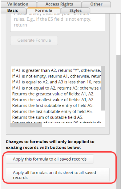
In some cases, you may need to recalculate a formula on all previous entries. To do so, you can choose to apply the formula change to all saved records, or, if you have modified more than one formula, apply all formulas on this sheet to all saved records.
Remember to save the design first before recalculating formulas in Design Mode.
Besides manually applying formula recalculation, you can also recalculate through the Workflow. Additionally, if you frequently change formulas or use TODAY(), you may consider using Daily Workflow to recalculate formulas daily.
Note: With workflow formula recalculation, there are two situations where changes will not be recorded in the entry history.
1. No changes are made after recalculation.
2. To optimize system performance, recalculations exceeding 3,500 entries will not be logged in the history (although the recalculation still executes normally).
To run a formula recalculation on related records on other sheets, go to Form Settings > Form Settings > Recalculate all formulas on parent or related sheets.
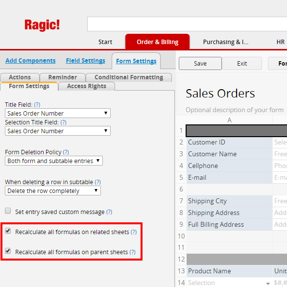
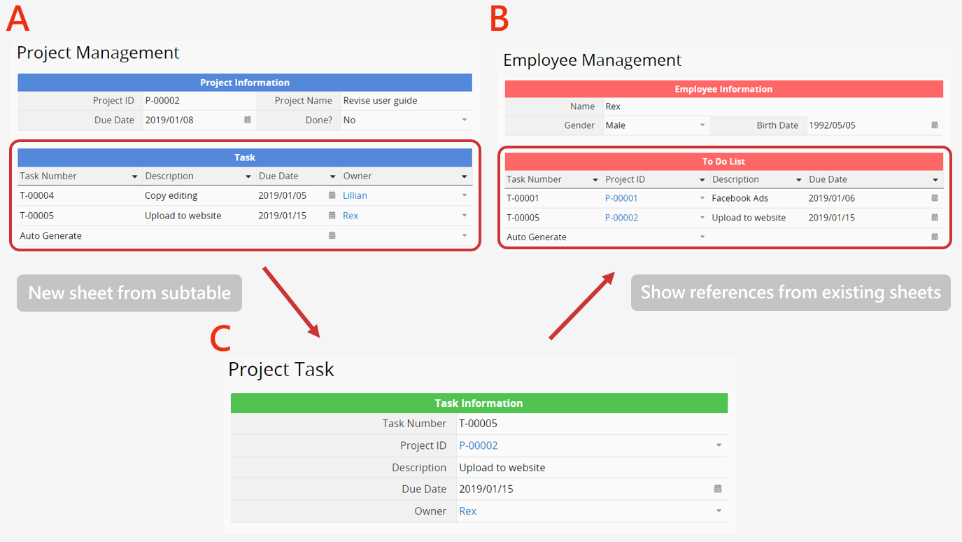
Parent Sheets:
In the above example, A and B are parent sheets of C.
Related sheets:
B and C are related sheets of A; A and C are related sheets of B.
Note: Currently, the limit number of recalculated records is 2000. If the number of records to be recalculated exceeds the system's limitation, it will ignore the setting to recalculate all formulas on related sheets.
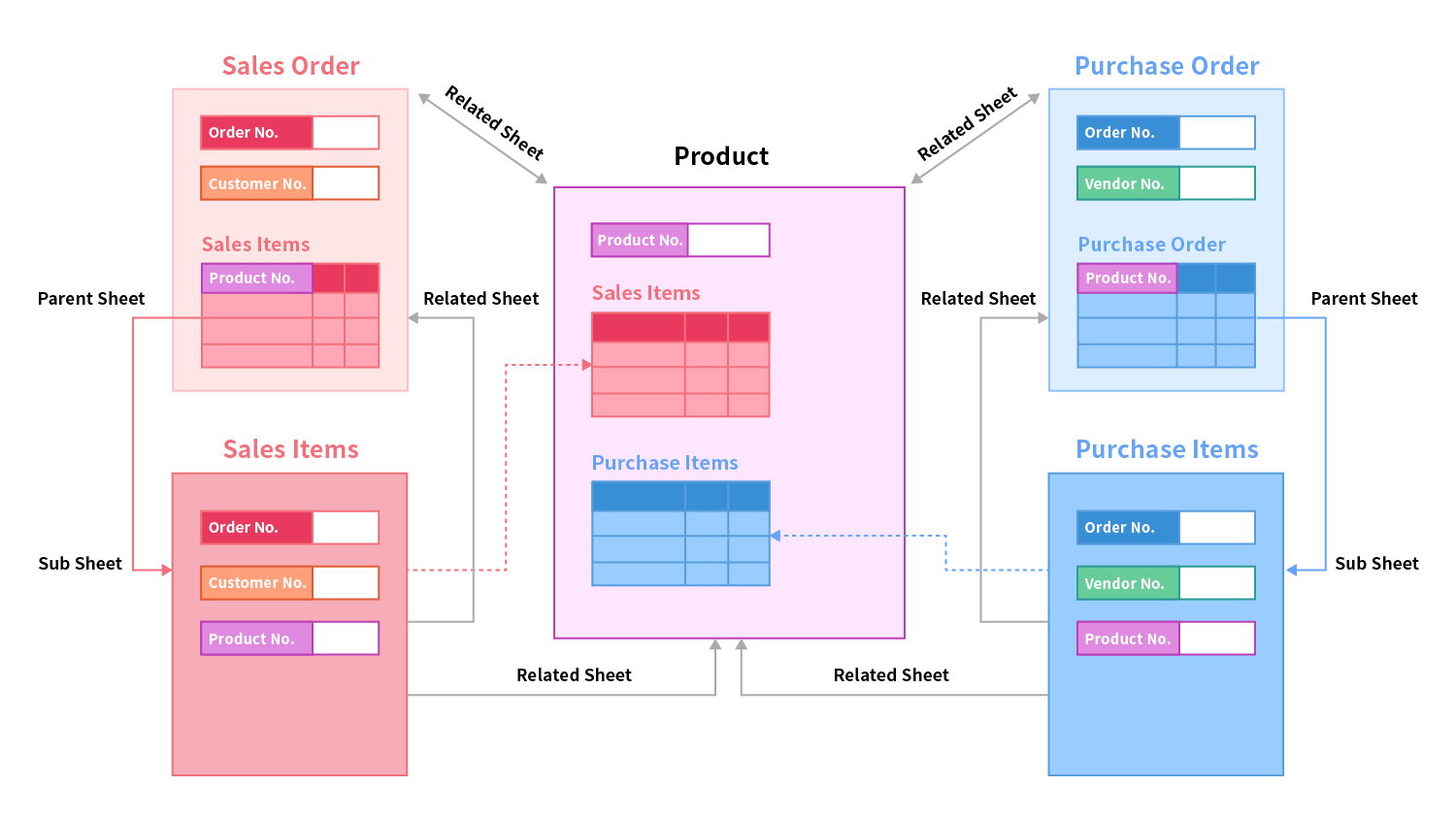
The diagram below shows the design concepts and logic between parent sheets, child sheets, and related sheets.
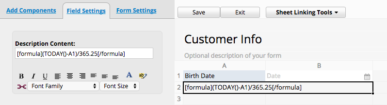
Formulas also work in Description Fields for display purposes only.
This is useful if you need to recalculate a formula each time your database form is loaded, but do not need to keep this value in your database. You will need to use the BBCode [formula] for your formula to work.
For example, to display a person's age based on their birthday, you can use the formula [formula](TODAY() - A1)/365.25[/formula] in a description field. This formula will continuously update to show the person's age according to the current date.
About the Math Objects supported in Ragic, please refer to this page.
If you need to use other unsupported formulas, please write to Ragic Support to suggest them.
 Thank you for your valuable feedback!